Copyright © 1999, 2002, 2007, 2024 Kees Krijnen.

Particle Sizing related Static, Dynamic and Electrophoretic LLS Instrumental Experiments

Laser light scattering (LLS) has provided an important method for particle sizing analysis for at least six decades [REF2]. Classical - static - light scattering (SLS) studies are concerned with the measurement of the intensity of scattered light by particles as a function of the scattered angle. In addition to this kind of study, spectral information can be obtained from the intensity fluctuations of scattered light - dynamic light scattering (DLS). Various forms of the latter type of experiment are known as light beating spectroscopy (LBS), intensity fluctuation spectroscopy (IFS), and photon correlation spectroscopy (PCS). PCS related experiments in laser doppler velocimetry (LDV) permit rates of uniform motion of particles to be measured. A special case of LDV is electrophoretic light scattering (ELS) where very low mobilities are determined.

Contents

• Introduction
• Digital Signal Processing
• Spectral Analysis
• One-dimensional Fast Fourier Transform
• Autocorrelation
• Photon Correlation Spectroscopy
• PALS Experimental Setup
• Results and Conclusion

Introduction

Today, applications of Digital Signal Processing (DSP) are numerous and still increasing rapidly every day. Typical DSP applications are CD music recording, modems, cellular phones, car ignition, electronic medical instruments, radar systems, etc. All these rely to some extent on digital signal processing [REF1]. DSP is based on representing signals by numbers in a computer (or in specialized digital hardware), and performing various numerical operations on these signals. The history of applied digital signal processing (at least in the electrical engineering world) began around the mid-1960 with the invention of the fast Fourier transform (FFT). However, its rapid development started with the advent of microprocessors in the 1970s. Early DSP systems were designed mainly to replace existing analog circuits, and did little more than mimicking the operation of analog signal processing systems. It was gradually realized that DSP has the potential for performing tasks impractical or even inconceivable to perform by analog means. Today, digital signal processing is a clear winner over analog processing.

Digital correlators have dominated dynamic light scattering experiments since their introduction in 1969. The analog signal from a light detector - generally a photo multiplier tube (PMT) - is digitized and processed further by digital hardware to extract the frequency shift signal from the noise. DSP microprocessors are generally too slow to process the digitized signal as it is produced for digital correlators, which is a digital pulse train of usually several MHz. However, DSP microprocessors can directly digitize the analog signal from a light detector and process it as a spectrum analyser or an analog correlator, or both simultaneously. Actually, before digital correlators became available these were the only techniques scientist could rely on to analyse dynamic light scattering by particles.

Digital correlators are almost entirely built from digital electronics and hardware - today even realized into one VSLI (very large-scale integration) chip. DSP microprocessors and systems are considered as digital hardware. However, their function and performance is totally based on embedded software engineering.

The objective of this web page is to give an instrumental overview - a compilation - of the application of DSP techniques in static and dynamic light scattering experiments. The theory of static, dynamic and electrophoretic laser light scattering is briefly reviewed. The experimental part of this web page starts with electrophoretic light scattering, a special case of dynamic light scattering, by means of spectrum analysis and `analog' autocorrelation. The signal - frequency shift - to be measured is well in the low area of the spectrum, 0-500Hz. No exceptional high DSP speed is required to process and analyze such a signal real-time. The measurements are setup as a phase analysis light scattering (PALS) experiment. The measurement principle of PALS and ELS are exactly the same.

Digital Signal Processing

The setup of a simple dynamic laser light scattering DSP system (fig.1) consist of:

• A conversion of a light detector analog signal into digital information, in the form of a sequence of binary numbers. This involves two operations: sampling and analog-to-digital (A/D) conversion.
• Perform numerical operations on the digital information by special-purpose digital hardware or PC. In this case the operations are spectrum analysis, "analog" autocorrelation, or both simultaneously.
• Display DSP process on PC monitor continuously.

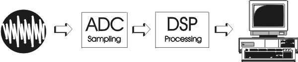
Fig. 1

To facilitate digital processing, a continuous-time signal must be converted to a sequence of numbers [REF1]. Sampling is essentially a selection of a finite number of data at any finite time interval as representatives of the infinite amount of data contained in the continuous-time signal in that interval. Sampling is the fundamental operation of digital signal processing, and avoiding (or at least minimizing) aliasing is the most important aspect of sampling. Aliasing is the fundamental distortion introduced by sampling. Aliasing causes the digitized pattern not look like the analog signal digitized. If analog signals at higher frequencies are present, the sampling process will produce sum and difference frequencies, in particular, will produce spurious low-frequency signals - in the signal passband - that cannot be distinguished from the signal. The Nyquist criterion provides a correct reconstruction of the analog signal, stated by Shannon's reconstruction theorem. Reconstruction is the operation of converting a sampled signal back to a continuous-time signal. Aliasing is caused by sampling at a lower rate than the Nyquist rate for the given signal.

Nyquist rate: sampling frequency ≥ 2 times highest frequency signal or noise component

Analog noise in data-acquisition systems take three basic forms [REF5]: transmitted noise, inherent in the received signal, device noise, generated within the devices used in data acquisition (preamps, converters, etc.), and induced noise, `picked up' from the outside world, power supplies, logic, or other analog channels, by magnetic, electrostatic, or galvanic coupling.

Noise is either random or coherent (i.e., related to some noise-inducing phenomenon within or outside the system). Random noise is usually generated within components, such as resistors, semiconductor junctions, or transformer cores, while coherent noise is either locally generated by processes, such as modulation/demodulation, or coupled-in. Coherent noise often takes the form of `spikes', although it may be of any shape.

The finite resolution of the A/D conversion process introduces `quantization noise', which may be thought of as either a truncation (or roundoff) error, or as a `digitizing' noise, depending on the context.

Noise is characterized in terms of either root-mean-square (rms) or peak-to-peak measurements, within a stated bandwidth. Noise leads to random errors and missing codes in an ADC. Since these errors can lead to a closed-loop system making inappropriate responses to specific false data points, high-resolution systems, where random noise tends to limit resolution and to cause errors, can benefit by digital or analog filtering to smooth the data.

If higher frequencies signal or noise than the Nyquist rate are part of the analog signal, a low-pass filter must be applied to match the Nyquist criterion.

Spectral Analysis

The departure point for a discussion of spectral analysis is the Fourier transform equation pair [REF5]:

Fourier Transform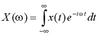

Inverse Fourier Transform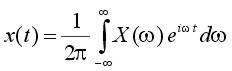

where t is time, ω is angular frequency (2πf), x(t) is the signal - a function of time - and X(ω) is its counterpart in the frequency (spectral) domain. These equations give us, at least formally, the mechanics for taking a signal' time-domain representation and resolving it into its spectral weights - called Fourier coefficients. The Fourier series is a trigonometric series F(f) by which we may approximate some arbitrary function f(t) or x(t) - real world signal [REF3]. Specifically, F(f) is the series (another way to describe above frequency-domain function X(ω)):

F(t) = A0 + A1Sin(t)+ B1Cos(t) + A2Sin(2t) + B2Cos(2t) + ... + AnSin(nt) + BnCos(nt)

e^iωt = Cos(ωt) + iSin(ωt)

In the limit as n (i.e. the number of terms) approaches infinity, the trigonometric series is equal to the real world signal. It means that any real world signal can be considered as a composite waveshape which can be breaked down into its component sinusoids. A0, A1, B1, ...and An, Bn, are the Fourier coefficients. When the Fourier coefficients are known the time-domain function x(t) can be easily calculated - reconstructed - by summation of the component sinusoids. Since the Fourier equations require continuous integrals, they have only indirect bearing on digital processors. However, under certain circumstances, a sampled (digitized) signal can be related faithfully to its Fourier coefficients through the discrete Fourier transform (DFT):

(Forward) DFT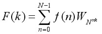

Inverse DFT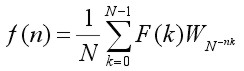

where:

F(k) = frequency components or transform f(n) = time base data points or inverse transform N = number of data points n = discrete times, 0 to N-1 k = discrete frequencies, 0 to N-1 WN = e-i2π/N = Cos(2π/N) - iSin(2π/N)

Provided that the signal is sampled frequently enough (Nyquist rate), and assuming that the signal is periodic, the above DFT equations hold exactly. What is most interesting from the standpoint of DSP is that the DFT equation provides us with a means to estimate spectral content by digitizing an incoming signal and simply performing a series of multiply/accumulate operations.

A process is required that can isolate, or `detect' any single harmonic (sine wave) component within a complex waveshape [REF3]. To be useful quantitatively, it will have to be capable of measuring the amplitude and phase of each harmonic component. While measuring any harmonic component of a composite wave, all of the other harmonic components must be ignored.

According to Fourier the way to detect and measure a sine wave component within a complex waveshape is to multiply through by a unit amplitude sine wave of the identical frequency and then find the average value of the resultant. The two functions must have the same number of data points, corresponding domains, etc. The reason this works is that both sine waves are both positive at the same time, and both negative at the same time, so that the products of these two functions will have a positive average value. Since the average value of a sinusoid is normally zero, the original digitized sine wave has been `rectified' or `detected'. This scheme will work for any harmonic component, changing the frequency of the unit amplitude sine wave to match the frequency of the harmonic component being detected. The same approach will work for the cosine components if the unit sine function is replaced with a unit cosine function.

Orthogonality is the method used to extract the sinusoid being analyzed while ignoring all other sinusoidal components [REF4]. Orthogonality implies that if one sinusoidal is multiplied by another, an average value of zero will obtained (averaged over any number of full cycles), if either:

1. the sinusoids are dephased by 90° or,
2. the sinusoids are integer multiple frequencies.

It is necessary to deal with full cycles of a sinusoid for the average value to be zero. This requirement can be satisfied by scaling the frequency term so that exactly one full sinusoid fits into the domain of the function working with.

The composite waveform is generated by summing in harmonic components:

F(t) = A0 + A1Sin(t)+ B1Cos(t) + A2Sin(2t) + B2Cos(2t) + ... + AnSin(nt) + BnCos(nt)

If this composite function is multiplied by Sin(Kt) (or, alternatively, Cos(Kt)), where K is an integer, the following terms on the right hand side of the equation are created:

A0Sin(Kt) + A1Sin(t)Sin(Kt) + B1Cos(t)Sin(Kt) + ... + AkSin2(Kt) + BkCos(Kt)Sin(Kt) + ... + AnSin(nt)Sin(Kt) + BnCos(nt)Sin(Kt)

Treating each of these terms as individual functions, if argument (Kt) equals the argument of the sinusoid it multiplies, that component will be `rectified'. Otherwise, the component will not be rectified. From what is shown above, two sinusoids of ± 90° phase relationship (i.e. Sine/Cosine), or integer multiple frequency, represent orthogonal functions. As such, when summed over all values within the domain of definition, they will all yield a zero resultant (regardless of whether they are handled as individual terms of combined into a composite waveform). This is precisely what is demanded from a procedure to isolate the harmonic components of an arbitrary waveform.

The DFT algorithm consist of stepping trough the digitized data points of the input time-domain function, multiplying each point by sine and cosine functions, and summing the resulting products into accumulators (one for the sine component and one for the cosine). When every point has been processed in this manner, the accumulators (i.e. the sum-totals of the preceding process) is divided by the number of data points. The resulting quantities are the average values for the sine and cosine components at the frequency being investigated as described above. This process must be repeated for all integer multiple frequencies up to the frequency that is equal to the sampling rate minus 1 (i.e. twice the Nyquist frequency minus 1).

If the digitized matrix f(t) is considered to be a row matrix, the process can be described as a matrix multiplication [REF6,7]:

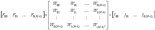
WN = e^-i2π/N = Cos(2π/N) - iSin(2π/N)

The DFT WNN square coefficient matrix is called the array of Twiddle Factors. One is needed for the Sine function and one for the Cosine function.

Unfortunately, the large number of multiplications required by the DFT limits its use in real-time signal processing. The computational complexity of the DFT grows with the square of the number of input points; to resolve a signal of length N into N spectral components F(k) requires N² complex multiplications (4N² real multiplications). Given the large number of input points needed to provide acceptable spectral resolution, the computational requirements of the DFT are prohibitive for most applications. For this reason, tremendous effort was devoted to developing more efficient ways of computing the DFT. This effort produced the fast Fourier transform (FFT) invented by Cooley and Tukey (1965). The FFT uses mathematical shortcuts to reduce the number of calculations the DFT requires.

The DFT (and FFT) requirement to deal with full cycles of a sinusoid rises inevitably the need for a high-pass filter. The frame length and timing of data acquisition determines the low cut-off frequency. The Nyquist criterion requires a low-pass filter, under experimental conditions this means a band-pass filter has to be applied to the input signal.

One-Dimensional FFT

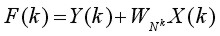
Suppose an N-point DFT is accomplished by performing two N/2 -point DFTs and combining the outputs of the smaller DFTs to give the same output as the original DFT. The original DFT requires N² complex multiplications and N² complex additions. Each DFT of N/2 input samples requires(N/2)² = N²/4 multiplications and additions, a total of N²/2 calculations for the complete DFT. Dividing the DFT into two smaller DFTs reduces the number of computations by 50 percent. Each of these smaller DFTs can be divided in half, yielding N/4 -point DFTs. If we continue dividing the N-point DFT calculation into smaller DFTs until we have only two-point DFTs, the number of complex multiplications and additions is reduced to Nlog2N. For example, a 1024-point DFT requires over a million complex additions and multiplications. A 1024-DFT divided down into two-point DFTs needs fewer than ten thousand complex additions and multiplications, a reduction of over 99 percent!

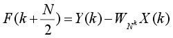
Dividing the DFT into smaller DFTs is the basis of the FFT. A radix-2 FFT divides the FFT into two smaller DFTs, each of which is divided into two smaller DFTs, and so on, resulting in a combination of two-point DFTs. The radix-2 Decimation-In-Time (DIT) FFT divides the input time-domain sequence into two groups, one of even samples and the other of odd samples. N/2-point DFTs are performed on these sub-sequences, and their outputs are combined to form the N-point DFT

The input time-domain sequence in equation (1), is divided into even and odd sub-sequences to become the equation:

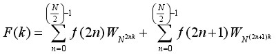(2)

By substitution equation (2) becomes:

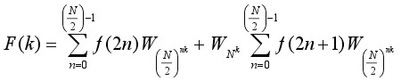(3)

By substitution equation (3) can also be expressed as two equations:

(4.1)

(4.2)

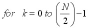
Together these equations (4.1) and (4.2) form an N-point FFT. Each of these two equations can be divided to form two more. The final decimation occurs when each pair of equations together computes a two-point DFT (one point per equation). The pair of equations that make up thetwo-point DFT is called a radix-2 `butterfly' (fig. 2). The butterfly is the core calculation of the FFT. The entire FFT is performed by combining butterflies in patterns determined by the FFT algorithm based on the Similarity, Shifting, Addition and Stretching transform theorems. An array of 2ⁿ data points yields n stages of computation in FFT.

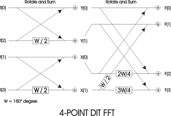
fig. 2

In general, the input of FFTs are assumed to be complex. When input is purely real - for example, in case of digitized analog data - their symmetric properties compute the DFT very efficiently [REF9].

One such optimized real FFT algorithm is the packing algorithm. The original 2N-point real input sequence is packed into an N-point complex sequence. Next, an N-point FFT is performed on the complex sequence. Finally the resulting N-point complex output is unpacked into the 2N-point complex sequence, which corresponds to the DFT of the original 2N-point real input.

Using this strategy, the FFT size can be reduced by half, at the FFT cost function of N operations to pack the input and unpack the output. Thus, the real FFT algorithm computes the DFT of a real input sequence almost twice as fast as the general FFT algorithm.

The TMS320C542 (see PALS Experimental Setup chapter) real FFT algorithm is a radix-2, DIT DFT algorithm in four phases:

In phase 1 - packing and bit-reversal of real input - the input is bit-reversed so that the output at the end of the entire algorithm is in natural order. First, the original 2N-point real input sequence is copied into contiguous sections of memory and interpreted as an N-point complex sequence. The even-indexed real inputs form the real part of the complex sequence and the odd-indexed real inputs form the imaginary part. This process is called packing. Next, this complex sequence is bit-reversed and stored into the data processing buffer.

In phase 2 - N-point complex FFT - an N-point complex DIT FFT is performed in place in the data-processing buffer. The twiddle factors are in Q15 format and are stored in two separate tables, pointed to by sine and cosine. Each table contains 512 values, corresponding to angles ranging from 0 to almost 180 degrees. The indexing scheme used in this algorithm permits the same twiddle tables for inputs of different sizes.

Phase 3 - separation of odd and even parts - separates the FFT output to compute four independent sequences, which are the even real, odd real, even imaginary, and the odd imaginary parts.

Phase 4 - generation of final output - performs one more set of butterflies to generate the 2N-point complex output, which corresponds to the DFT of the original 2N-point real input sequence.

Often, the last stage in a FFT spectral analysis is the computation of the power spectrum from the frequency-domain transform of the input time-domain sequence.

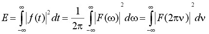
The power spectrum is a meaningful way of representing random signals in the frequency domain by their mean-square value or energy content. Now from Parseval's theorem [REF10]:

(5)

where ω = 2πν and ν is expressed in Hertz. Equation (5) states that the energy content of f(t) is given by 1/(2π) times the area under the |F(ω)|² curve. For this reason, the quantity |F ω)|² is called the power spectrum or energy spectral density of f(t).

Autocorrelation

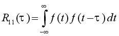
Autocorrelation gives an indication to what degree the time signal f(t) is similar to a displaced (delayed) version of itself as a function of the displacement. This technique is - for example - used for the detection of echoes in the signal (radar, sonar) or detection of periodic signals buried in random noise (LDV, ELS). The autocorrelation function is defined by [REF10]:

(6)

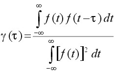
Sometimes, a normalized quantity γ(τ) defined by

(7)

is also called the autocorrelation function of f(t). In this case it is clear that γ(0) = 1. The average autocorrelation function of periodic signals of period T are also periodic with the same period. This does not mean that autocorrelation function of a periodic signal will have the same waveshape as the signal autocorrelated. The autocorrelation of a sine wave is a cosine waveshape [REF10]. This means when looking for a periodic sinusoid signal in random noise the autocorrelation function will show a cosine waveshape mixed with the autocorrelation function of the random noise.

The basics of a digital hardware correlator are shown by means of reviewing an existing correlator IC device from TRW LSI Products Inc. (fig. 3). This device has been designed not only for auto- or crosscorrelation, but also for pattern and character recognition, video frame synchronization, bar code identification, radar signature recognition etc.

The TRW TMC2023 is an monolithic 64-bit correlator with a 7-bit three-state buffered digital output. This device consist of three 64-bit independently clocked shift registers, one 64-bit reference holding latch, and a 64-bit independently clocked digital summing network. The device is capable of a 30MHz parallel correlation rate.

The 7-bit threshold register allows the user to preload a binary number from 0 to 64. Whenever the correlation is equal to or greater than the number in the threshold register, the threshold flag goes HIGH.

The 64-shift mask register (M register) allows the user to mask or selectively choose `no compare' bit positions enabling total word length flexibility. In case of autocorrelation this mask register is used for the undelayed clocked signal.

The summing process is initiated when the comparison result between the A register and R latch (NXOR-gate) is clocked into the summing network by a rising edge of CLK S. Typically, CLK A and CLK S are tied together so that a new correlation score is computed for each new alignment of the A register and the R latch. Every clock cycle the contents of register n is shifted to register n+1. When LDR goes HIGH, the contents of register B are copied into the R latch. With LDR low, a new template may be entered serially into register B, while parallel correlation takes place between register A and the R latch.

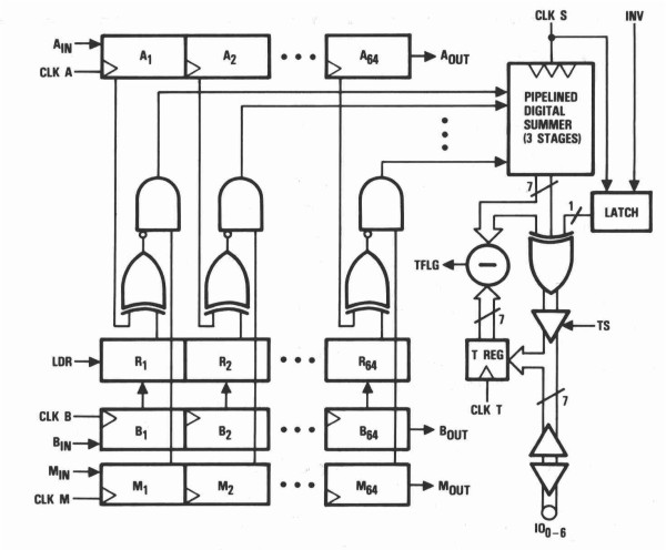
fig. 3. Functional block diagram TMC2023 (courtesy TRW LSI Products. Inc.).

In case of a 1x1-bit autocorrelator function, shift registers B and M - tied together - are used for the undelayed signal. CLK A, CLK B, CLK M and CLK S are also tied together. Input A_IN is held HIGH, filling register A with ones. Every clock cycle B_IN and M_IN are shifted into B₁ and M₁, and register B_n and M_n are shifted into B_n+1 and M_n+1. Every 64-clock cycles register B is copied into the R latch by a LDR HIGH pulse - an external clock counter circuit is needed, which resets every 64-clock cycles and gives the LDR pulse. After this copy action latch register R is n clock cycles delayed compared to register M until the clock counter equals 64, loads register B into the R latch, and resets again. The AND-gate acts as a 1x1-bit multiplier of register R (delayed B) and M, multiplication - equation (6) - is required. The output IO_0-6 gives the summing of the 64-channel 1x1-bit autocorrelation every clock cycle of the delayed signal.

A microprocessor keeps track of the autocorrelation process over multiple 64-clock cycles. Every clock cycle the microprocessor reads the summing result IO_0-6 and the contents of the clock counter. The summing result is added to an array indexed by the clock counter. This array gives the integrated 64-channel 1x1-bit autocorrelation function over a finiteperiod of time.

The scheme for a nxn multi-bit autocorrelator is exactly the same. The shift registers are n multi-bit shift registers. The latch register is a n multi-bit latch register. Instead of an AND-gate a nxn multiplier device is required.

The first PCS autocorrelators were 1x1-bit correlators. Ideally the PMT light detector electronics generates one digital pulse for each photon the PMT receives what makes the light detection truly digital. The 1x1-bit correlators were perfectly suited to correlate the PMT digital pulse train. However, this meant that the autocorrelation clock rate should be higher or equal to the digital pulse rate. In practice this requirement is not easily achieved. The correlation clock rate - sample time - is set to a value to maximize autocorrelation resolution. If more than one pulse is received within the sample time overflow occurs. Prescaling or multi-bit correlation avoids clipping of the digital input signal. Nowadays, PCS autocorrelators are multi-bit correlators allowing prescaling if necessary, offer multiple simultaneous correlation sample times, or even logarithmic sample times.

The implementation of autocorrelation by means of a DSP microprocessor is almost directly derived from equation (6). A frame of N data points is acquired continuously and stored into a circular buffer of size N. The last acquired data point overwrites the first - oldest - one. Between successive samples, the last acquired data point - f(0) - is multiplied with itself and with the previous N-1data points. The multiplication results are added to an array of size N, indexed by the number of data points difference between the last data point and the previous N-1 data points. The array contents indexed by 0 to (N-1) gives the integrated autocorrelation function.

To find a periodic signal burried in the signal f(t), the Fourier transform of the autocorrelation function is computed, which is called the energy spectrum density of f(t). If f(t) is a real function, then the autocorrelation function R₁₁(τ) and the energy spectral density |F(ω)|² constitute a Fourier transform pair [REF10]; that is,

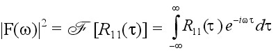(8)

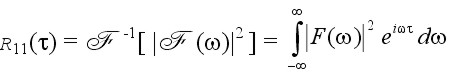
This result is known as the Wiener-Khintchine theorem.

The number of autocorrelation channels of a DSP microprocessor correlator is limited by the time available for the multiplication process between successive samples. If the energy spectrum is computed simultaneously - by means of FFT - the time available, and so the number of autocorrelation channels is even more limited. Another restricting factor is that the FFT computation requires a log₂ number of data points. It limits the autocorrelation resolution by forcing the number of autocorrelation channels also bound to log₂, even if there is computation time left to setup more autocorrelation channels.

Photon Correlation Spectroscopy

Classic - static - light scattering is concerned with the average intensity of the scattered light and its dependence on both the concentration and size of scattering particles, and the scattering angle. The intensity of scattered light depends inverse fourth power on wavelength (Raleigh, 1871) and sixth power on radius of particle.

For particles less than ¹/₁₀th of wavelength of the illuminating beam, the scattering is isotropic, equal energy is scattered at all angles - Raleigh theory. Mie theory (1908) describes exactly how particles of different sizes and optical properties interact with light and is used to analyze light scattering of particles above ¹/₁₀th of wavelength. Mie theory approximation computing algorithms have an upper limit due to (optical parameter) ill-conditioning [REF11]. Above this limit Anomalous Diffraction and Fraunhofer Diffraction approximations [REF12] can be used. References [REF11], [REF12] and [REF13] are excellent, comprehensive papers on static light scattering by particles.

Intensity Fluctuation Spectroscopy - dynamic light scattering - is concerned with the amplitude modulation of the scattered light. In case of an illuminated suspended sample, the modulation is caused by interference of scattered light due to the Brownian movement of the suspended particles. Brownian motion (Brown, 1828) is the random movement of suspended particles due to collision with the random thermal motion of solvent molecules (Einstein, 1905). If the suspended particle is big compared to the solvent molecules those movements will be small. Smaller particles will move faster, due to the greater influence of the solvent molecules.

Interference occurs because of the different path lengths traversed by light scattered from different particles. The illuminating beam must be coherent, that means light waves must be parallel and in phase. Lasers produce coherent, monochromatic light. The temporal fluctuations of interest appear in one coherence area, and the signal-to-noise ratio does not increase when more than one coherence area is detected. The intensity of a coherence area will be seen to vary as dark and light patches interchanging in the field of view. The rate of these fluctuations is determined by the speed of the diffusing particles - related to particle size, shape, and medium viscosity and temperature.

A coherence area could be defined as the coherently illuminated minimum volume resulting maximum intensity modulation by interference. Intensity modulation will minimize - intensity of scattered light becomes constant - when the viewed area is too large (incoherent). Ideally, one coherence area is viewed, depending on quality of optics and sensitivity of light detector.

The rate of the intensity fluctuations vary with speed of diffusing particles and are random, no distinctive sinusoid can be detected. Although, autocorrelation does not extract sinusoids from the intensity fluctuations, the correlatorgram shows an exponential curve. The rate of decay is related to the diffusion coefficient of the suspended particles. Autocorrelation detects similarity of the scattering signal in time, and this similarity will be lost sooner when particles move faster - are smaller - thus resulting a faster decay of the exponential correlation curve.

Generally, a photon multiplier tube (PMT) is used as a light detector. These are photo emissive devices coupled with electron multipliers. When a photon strikes the photocathode, an electron is emitted and multiplied by sequential dynodes. The multiplier sections have typical gains of 10⁶ so that a measurable current is produced at the anode. In a photon counting system the pulses resulting from - ideally single - photons are selected, amplified and correlated, hence the name Photon Correlation Spectroscopy (PCS).

The autocorrelation of the scattered electric field E of the incident light and the frequency components of the intensity signal form a Fourier transform pair - equation (8). When the autocorrelation of E is known, the frequency components can be computed. Detectors, e.g. PMTs, respond to the intensity I rather than the electric field of incident light. In general, the autocorrelation of I [G₂(τ) - second order] is not simply related to autocorrelation of E [G₁(τ) - first order]; however, if E(t) is a Gaussian random variable the Siegert relation gives

G₂(τ) = I ² + |G₁(τ)|²

By substitution the normalized second order autocorrelation function becomes

G₂(τ) = 1 + Ce^-τt (9)

where:

τ = 2DτK2 C = experimental constant correlator Dτ = diffusion coefficient K = λ = wavelength of laser Φ = scattering angle n = refractive index suspending liquid

Gaussian random means that the number of particles contributing to the intensity modulation of scattered light should be significant and Gaussian distributed. In experimental conditions this viewed number should be at least one hundred. The Stokes-Einstein equation for diffusion of a monosized sample states:

D_τ =

where:

k = Boltzmann's constant T = absolute temperature η = viscosity of the solvent d = spherical particle diameter

Thus, using PCS, average size of monodispersed spherical samples can be determined based on first principles. The size distribution determination of polydispersed samples is a lot more difficult; (1) different polydisperse size distributions can give similar autocorrelation results, and (2) intensity depends sixth power on radius, bigger particles contribute more to the signal than smaller ones. A more extensive treatment of PCS theory can be found in reference [REF2].

Frequency determination for light scattered from particles in uniform motion are conceptually simpler than for diffusing particles. Laser Doppler Velocimetry (LDV) is a well established technique in engineering for the study of fluid flows. Two laser beams in phase are caused to cross at a particular point in the measurement cell. The lens in the receiver optics - a coherent detector - is focussed at the center of this crossing point. At the intersection of the laser beams, Young's [REF14] interference fringes are formed of known spacing given by the simple equation

(10)

Particles moving through this fringe pattern scatter light what gives rise to a sinusoidal intensity modulation at the detector whose frequency can be measured and thus the related velocity calculated by multiplying S with found frequency. The frequency is determined by a Fourier transform - equation (8) - of the autocorrelation function, which also gives the autocorrelation due to scattered light by the Brownian movement of suspended particles. The latter autocorrelation function is, in respect to LDV, background noise.

The following experiment is setup as a LDV experiment. The results can be applied to Electrophoretic Light Scattering (ELS). The essence of an ELS system is a cell with electrodes at either end to which a potential gradient is applied. Charged particles move towards the appropriate electrode through the crossing point of the laser beams, their velocity is measured and expressed in unit field strength as their mobility. The stability of suspended particles, emulsions, are strongly influenced by the electrical charges that exist at the particle liquid surface.

The term Laser Doppler Velocimetry is - however in the past established in publications like [REF2] - not a correct description of the physical phenomena. LDV was originally setup as a low angle single laser beam experiment where the laser beam crossed high speed particles like those ejected out of a jet fighter exhaust. Those high speed particles indeed caused a doppler shift of the laser light frequency. When two laser beams in phase were crossed the same term was still used, however in this case for low speed particles the sinusoidal intensity modulation delivers the information. The term Phase Analysis Laser Scattering (PALS) is applied when one of the laser beams is modulated.

PALS Experimental Setup

The experimental setup consist of (fig. 4) :

• Helium-Neon laser, wavelength 632.8 nm, to provide a coherent light source
• Beam expander and focus optics, to maximize scattering at crossing point
• Beam splitter and two mirrors to generate two equal laser beams in phase
• Glass tube at the crossing point of the two laser beams to measure sample
• Coherent detector - 200 µm pinhole, objective focus lens, 2nd pinhole and phototransistor
• AC amplifier to amplify intensity modulation from detector
• TMS320C542 DSP evaluation board with ADC
• 486 PC (DOS/WIN3.11) to monitor process and save data

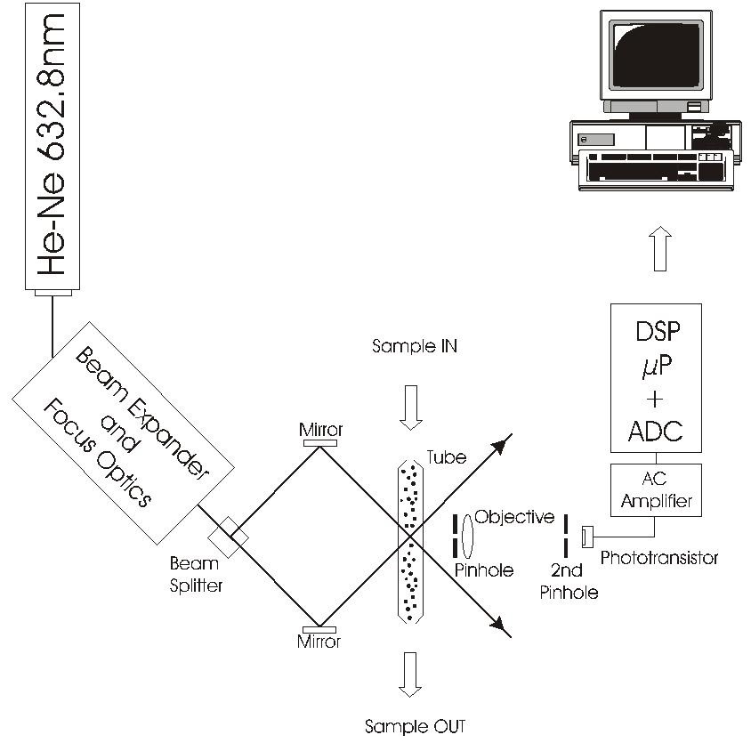
fig. 4. PALS Experimental setup.

The laser is a 5mW HeNe polarized laser from Melles-Griot, Carlsbad CA, USA. It requires a high voltage power supply (1.85-2.45kV, 6.5mA).

The tube is a cilindrical glass capillary, inner diameter 4 mm. The angle between the two laser beams, inside the tube, is affected by the difference in refractive index of medium inside and outside tube - Snell's law [14]. Sample is transported from reservoir to capillary via silicon tubes, and afterwards to waste.

Creamer solved in tap water has been used as test sample for PALS experiments, what provides a stable suspension. The concentration is chosen in such a way that the laser beams are clearly visible, there is no `glowing cloud' around the beams. As liquid transportation, gravity is used. The waste is lower than the sample reservoir. By varying the height of waste in respect to reservoir, different liquid flows can be set.

Instead of a photo multiplier tube a phototransistor is selected from UDT Sensors Inc., Hawthorne CA, USA. No specifications are known, but this phototransistor was applied in a system where extremely high sensivity for light was required

The AC amplifier allows amplification from 1x to 500x to be selected by jumpers. The lower power supply ±5V of driver stage is meant to prevent overloa of the ADC input; 6V differential load is allowed. OPA77 opamps were used, instead of OPA90. OPA90 is better suited for low power supply applications, but was not available. The driver stage OPA77 opamp shows some clipping for high negative outputs, but this has not affected results.

The TMS320C542 evaluation board (fig. 5) with TLC320AC01 14-bit ADC processes the signal from AC amplifier board. This DSP starter kit from Texas Instruments Inc. is supplied with DSKplus development board, C54x algebraic assembler, GoDSPs WindowsTM-based Code ExplorerTM debugger and various application programs.

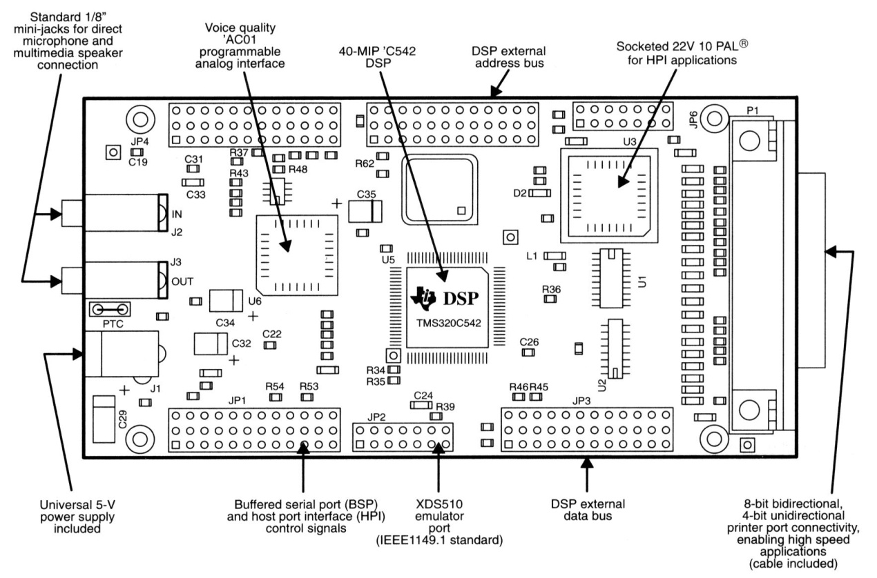
fig. 5. DSKplus Board Diagram (courtesy Texas Instruments Inc.)

Several features of the DSKplus board enable MIPS-intensive, low-power applications:

• One TMS320C542 enhanced fixed point DSP
• 40 MIPS (25-ns instruction cycle time)
• 10K words of dual-access RAM (DARAM)
• 2K words boot ROM
• One time-division-multiplexed (TDM) serial port
• One host port interface (HPI) for PC-to-DSP communications
• Programmable, voice-quality TLC320AC01 (DAC, ADC interface circuit)

The host port interface is an on-board PAL® device that operates as the main interface between the host PC parallel port and the C542 host port interface (HPI). As a result, the interface logic gives the host PC direct control of the C542 HPI and DSP reset signal, and it can configure the board to operate with different PC parallel ports (that is, 4-bit and 8-bit printer ports).

The C542 (fig 6.) has a high degree of operational flexibility and speed. It combines an advanced modified Harvard architecture (with one program memory bus, three data memory buses, and four address buses), a CPU with application-specific hardware logic, on-chip peripherals, and a highly specialized instruction set. Key features of C542 CPU, memory and instruction set are:

• Advanced multibus architecture with one program bus, three data buses, and four address buses
• 40-bit arithmetic logic unit (ALU), including a 40-bit barrel shifter and two independent 40-bit accumulators
• 17-bit x 17-bit parallel multiplier coupled to a 40-bit dedicated adder for nonpipelined single-cycle multiply/accumulate (MAC) operations
• Compare, select, store unit (CSSU) for the add/compare selection of the Vertibi operator
• Exponent encoder to compute the exponent of a 40-bit accumulator value in a single cycle
• Two address generators, including eight auxiliary registers and two auxiliary registers arithmetic units. Circular indexed addressing
• On-chip 2K ROM and 10K DARAM memory
• Single-instruction repeat and block repeat operations
• Block memory move instructions for better program and data management
• Instructions with a 32-bit long operand
• Instructions with 2- or 3-operand simultaneous reads
• Arithmetic instructions with parallel store and parallel load
• Conditional store instructions
• Fast return from interrupt

Separate program and data spaces allow simultaneous access to program instruction and data, providing a high degree of parallelism. For example, three reads and one write can be performed in a single cycle. Instructions with parallel store and application-specific instructions fully utilize this architecture. In addition, data can be transferred between data and program spaces. Such parallelism supports a powerful set of arithmetic, logic and bit-manipulation operations that can all be performed in a single machine cycle. Also, the C542 includes the control mechanism to manage interrupts, repeated operations, and fuction calling.

Features most important for the experimental setup are single-cycle multiplication with indexed addressing, circular indexed addressing and MAC operations.

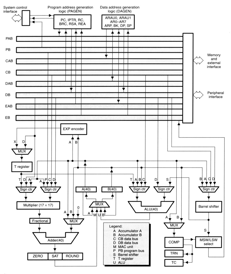
fig. 6. Block diagram C542 internal hardware (courtesy Texas Instruments Inc.)

The AC01 analog interface circuit (fig. 7) provides a single channel of voice-quality data acquisition. The AC01 has the following features:

• Single-chip solution A/D and D/A conversion with 14 bits of dynamic range
• Built-in, programmable antialiasing filter
• Software-programmable sampling rates
• Software-programmable reset, gain, and loopback
• Software-selectable auxiliary input
• 2nd-Complement 16-bit aligned Data Format

The AC01 interfaces directly to the C542 TDM serial port. The AC01 generates the required shift clock (SCLK) and frame sync (FS) pulses used to send data to/from the AC01. These pulses are a function of software-programmable registers and the AC01 master clock. The master clock (MCLK) is generated by the on-board 10 MHz oscillator.

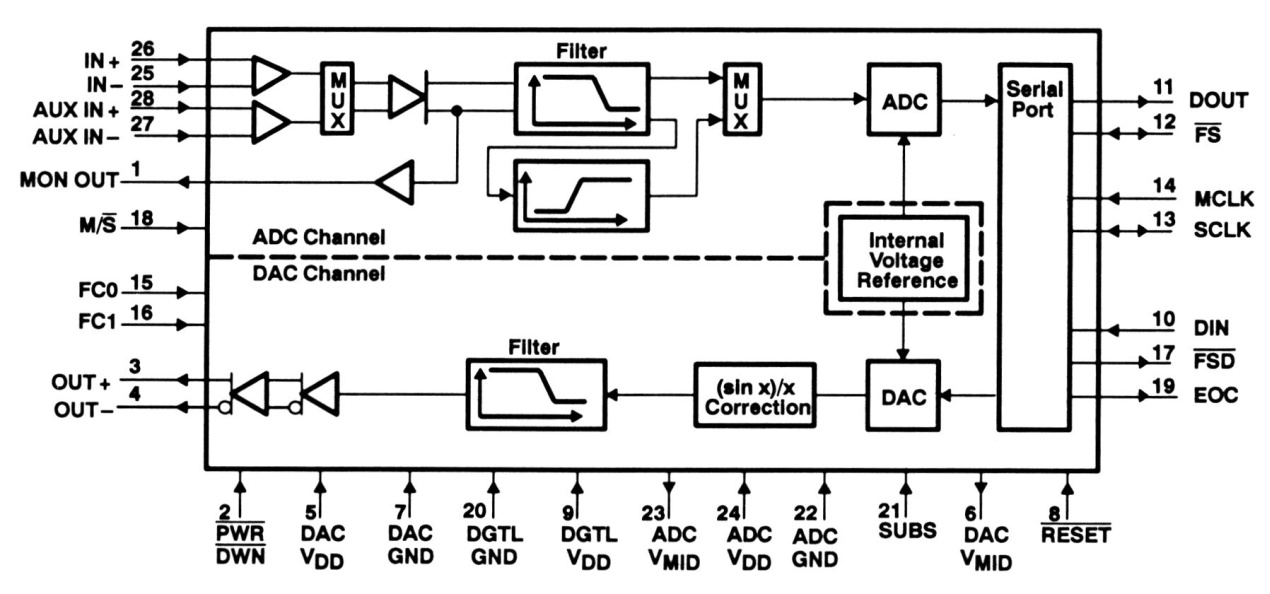
fig. 7. AC01 functional block diagram (courtesy Texas Instruments Inc.)

For convenient value reading a master clock (MCLK) of 10.368 MHz is assumed. All frequencies mentioned below and in Results chapter should be multiplied with ¹⁰/_10.368 to get their real value!

Sampling frequencies of 2 kHz, 4 kHz and 8 kHz are applied. Their respective low-pass and high-pass filter frequencies are (B register value is default 18):

2 kHz - f(LP) = 900 Hz, 4 kHz - f(LP) = 1800 Hz, 8 kHz - f(LP) = 3600 Hz,

f(HP) = 10 Hz, f(HP) = 20 Hz, f(HP) = 40 Hz,

AC01 A reg. = 144 AC01 A reg. = 72 AC01 A reg. = 36

The f(LP)s match the Nyquist criteria. The minimum aquisition frame length used is 256 data points. Dividing the sampling frequency with this number gives the lowest extractable frequency - see full-cycle DFT/FFT requirement. The f(HP)s match as well, for example ⁸⁰⁰⁰/₂₅₆ ± 31 Hz.

PALS Results and Conclusion

The objective of the experimental setup is to investigate the application of DSP in PALS experiments by means of implementation of a DSP microprocessor Spectrum Analyser, Autocorrelator and Energy Analyser.

The PC interface program implements a monitor to view the actual frame (oscilloscope function), the power (SA) or energy spectrum (AEA), and the autocorrelation function of power spectrum (SA) or integrated autocorrelation of actual frame (AEA). Another feature is to save what is displayed on screen. The applications are written in C542 algebraic assembler. The PC interface DOS program is written in C.

The same PC interface program is used for both applications. This means that for the Spectrum Analyser the Autocorrelation option displays the autocorrelation of the power spectrum to find significant frequencies - a limited number of power spectrum frames are computed. For the Autocorrelator and Energy Analyser application the Autocorrelation option displays the integrated autocorrelation of the aquisited frames, the Power Spectrum option is in fact the energy spectrum.

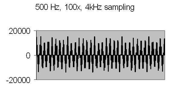
Results Spectrum Analyser

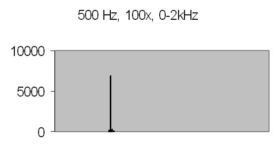
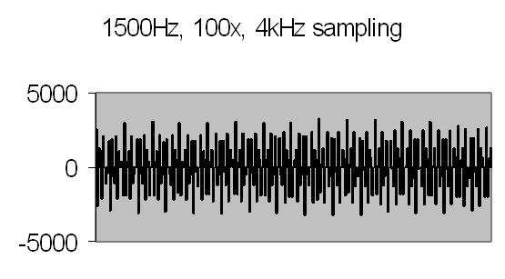
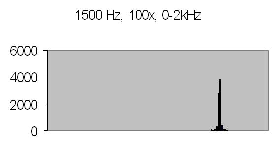
Figures 8 to 11 show the power spectrum of test signals from a Philips PM 5190 signal generator. Several positive sinoids are generated with a DC offset and applied to a light emmiting diode (LED). In this way the light detector is tested as well. The signals applied are the values listed, but the range of the power spectrum should be multiplied with ¹⁰/ _10.368 to get the actual value - see Experimental Setup chapter! The legend lists the signal applied (ADC value), the AC amplification and the power spectrum range.

fig. 8	fig. 9
fig. 10	fig. 11

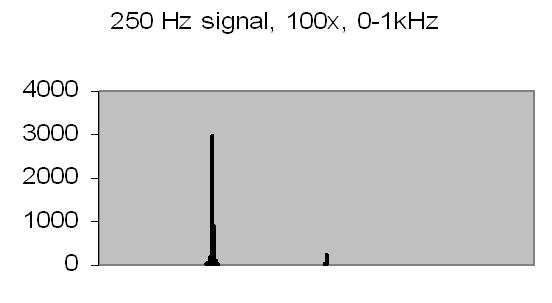
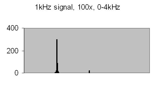
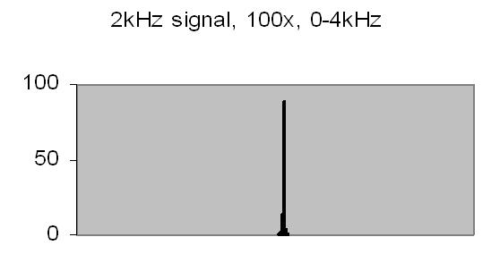
The upper limit of the power spectrum range is half the sampling frequency. For above examples a 2kHz and 8kHz sampling frequencies are applied. Figs. 8. and 10. also show the second harmonics. The energy content, the Y-axis (ADC value), drops from 3000 at 250Hz to 90 at 2kHz due to the higher frequency (less photons per sample).

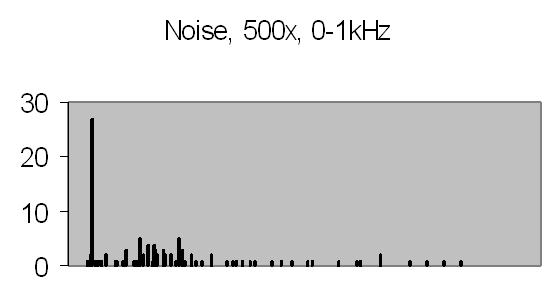
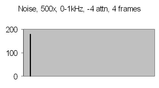
Figs. 12 and 13 show the 50Hz mains noise at an amplification of 500x - no light detected. Fig. 12 shows the power spectrum and fig. 13 the autocorrelation from four successive power spectrum frames. By autocorrelation of successive power spectra significant frequencies are found.

fig. 12. power spectrum

fig. 13. spectra autocorrelation

The test sample stopped flow signals, power spectra and autocorrelations are shown in figs. 14a, 14b, 15a, 15b, 16a and 16b. `A' and `B' are independent data aquisition frames.

Fig. 14a. Signal A	Fig. 14b. Signal B
Fig. 15a. Power spectrum A	Fig. 15b. Power spectrum B
Fig. 16a. Autocorrelation spectra A	Fig. 16b. Autocorrelation spectra B

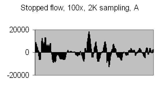
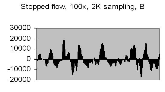
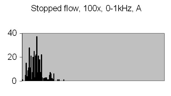
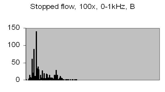
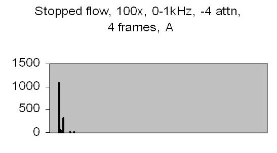
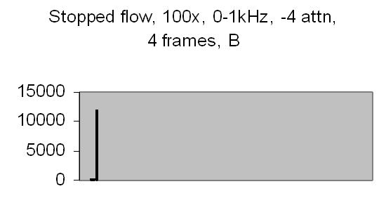
Figs. 14a to 16b show in fact the background noise due to the Brownian movement of the suspended particles. It's a random signal, it varies from frame to frame. Autocorrelation of four successive spectra show some significant frequencies, but as more spectra frames are autocorrelated no significant frequencies are expected.

Figs. 14a and 14b make clear that the phototransistor is sensitive enough to detect the light scattering by interference from the random moving suspended particles. The sensivity depends on AC amplification factor (100x) and surface area of light detector. The surface area of applied light sensitive detector is approximately 25mm². The internal amplification factor of the phototransistor is not known. The AC01 ADC has an input sensivity of ± 1.5V set. The signal figures also show that the dynamic range of ADC is properly used. The 14-bit ADC value in 16-bit 2nd complement format has limits from -32768 to 32767.

The test sample slow flow signals, power spectra and autocorrelation are shown in figs. 17a, 17b, 18a, 18b, 19a and 19b.

Fig. 17a. Signal A	Fig. 17b. Signal B
Fig. 18a. Power spectrum A	Fig. 18b. Power spectrum B
Fig. 19a. Autocorrelation spectra A	Fig. 19b. Autocorrelation spectra B

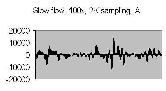
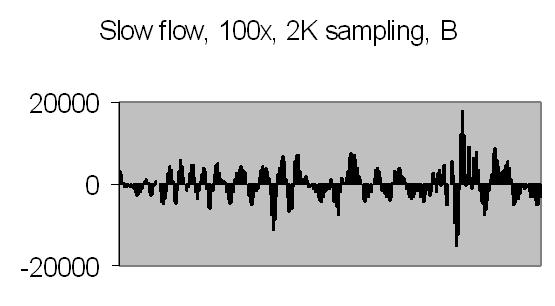
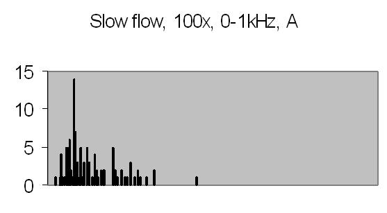
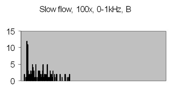
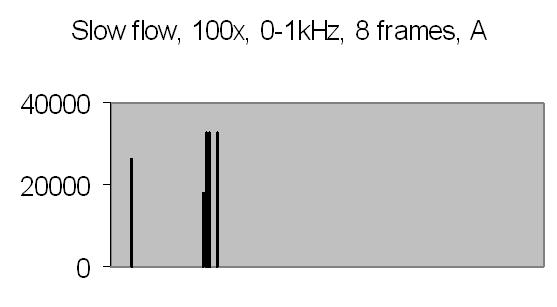
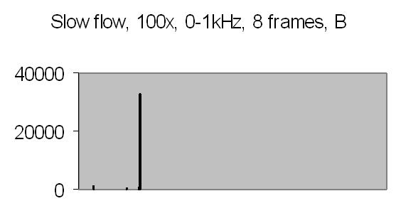
Figs. 19a and 19b compared to figs. 16a and 16b show that peaks found at 45-49Hz are caused by the Brownian movement of suspended particles. Fig. 19a peaks at 203-241Hz and fig. 19b peaks at 188-196Hz are peaks due to sinusoidal signal caused by suspended particles passing the dark and light bars of Young's fringes. Some peaks in the figs. of 19a and 19b are saturated, they are the result of multiplying eight power spectra. No attenuation is applied like figs. 16a and 16b (4 bit right shifting result after each multiplication).

It is difficult to avoid saturation. The energy content depends on the signal amplitude. This varies from frame to frame. Other concentrations or other samples will give different signal amplitudes, thus different power spectra. It will be difficult to set up a general attenuation and autocorrelation number of power spectra. The need for attenuation is a result from applying a fixed point DSP microprocessor - it has a limited dynamic range.

Another approach could be adding of all collected power spectra - saturation by adding will not happen as soon as saturation by multiplication. Unfortunately, this approach would also include all noise contributions. Autocorrelation is a tool to extract signal from noise.

Above signal figures are the first half (256 data points) from a frame of 512 data points. The power spectra are computed from a frame of 512 data points resulting a 256 points frame.

Results Autocorrelator and Energy Analyser

Figures 20a to 23b show the autocorrelation and energy spectra of test signals from a Philips PM 5190 signal generator - see results spectrum analyser - and a CEL213 random noise generator. The actual range of the energy spectra is ¹⁰/_10.368 the listed value - see Experimental Setup chapter! The random noise signals are directly applied to the ADC input.

Fig. 20a. Autocorrelation	Fig. 20b. Energy spectrum
Fig. 21a. Autocorrelation	Fig. 21b. Energy spectrum
Fig. 22a. Autocorrelation	Fig. 22b. Energy spectrum
Fig. 23a. Autocorrelation	Fig. 23b. Energy spectrum

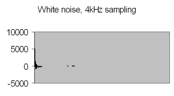
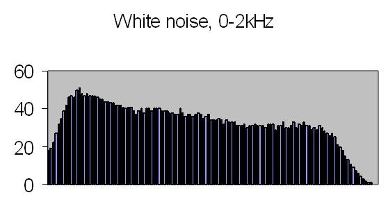
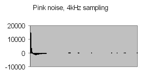
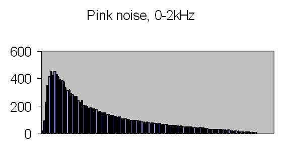
Figs. 20a to 23a show the continuous autocorrelation from a 256 data points signal frame. The Fourier transform - the energy spectrum - from the autocorrelation is given in figs. 20b to 23b. The latter result has 128 data points - half the data points of the autocorrelation frame.

The white noise signal autocorrelation, fig. 22a shows a fast decay to zero, what is expected from a true random signal - there is very little similarity in time. The white noise energy spectrum (fig. 22b) is affected by the bandwith filter. The tableau should be flat, theory predicts a constant energy for all frequencies, but results are acceptable. The pink noise energy spectrum displays an expected exponential curve (fig. 23b). The density is proportional to ¹/_f.

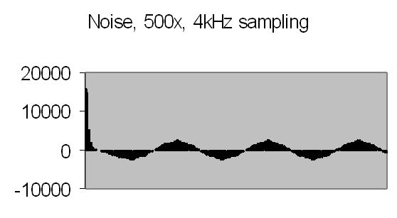
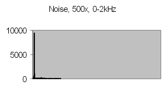
Figs. 24a and 24b show the 50Hz mains noise at an amplification of 500x - no light detected.

Fig. 24a. Autocorrelation

Fig. 24b. Energy spectrum

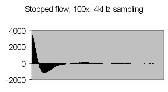
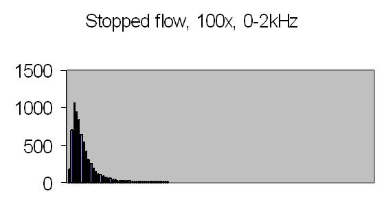
Figs. 25a and 25b display the results from a stopped flow signal. The PCS theory predicts a decaying exponential curve for monosized particles. However, for a broader (gaussian) particle size distribution the autocorrelation of the scattered light displays a decaying cosine.

Fig. 25a. Autocorrelation

Fig. 25b. Energy spectrum

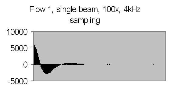
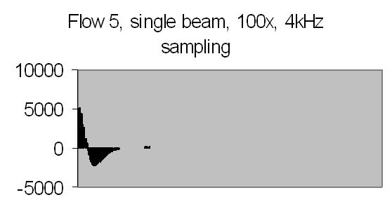
Figs. 26a to 30b show results from five different flows. Flow 1 is the slowest flow, increasing to the highest flow - flow 5. To be sure that the extra peak is produced by the passing of suspended particles through Young's fringes, a single beam result is collected as well - for example figs. 31a and 31b. A single beam result is exactly the same as a stopped flow result.

Fig. 26a. Autocorrelation	Fig. 26b. Energy spectrum
Fig. 27a. Autocorrelation	Fig. 27b. Energy spectrum
Fig. 28a. Autocorrelation	Fig. 28b. Energy spectrum
Fig. 29a. Autocorrelation	Fig. 29b. Energy spectrum
Fig. 30a. Autocorrelation	Fig. 30b. Energy spectrum
Fig. 31a. Autocorrelation	Fig. 31b. Autocorrelation

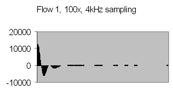
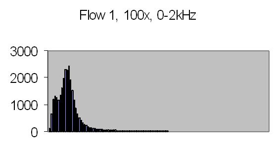
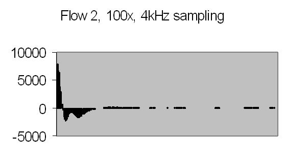
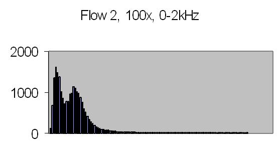
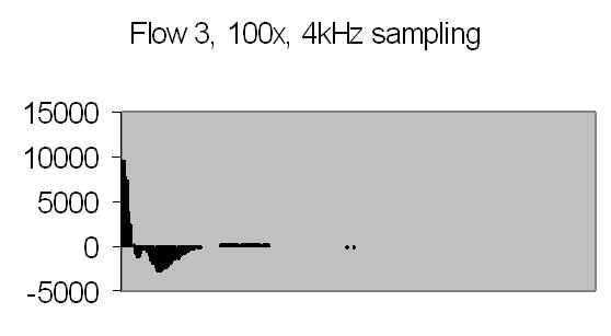
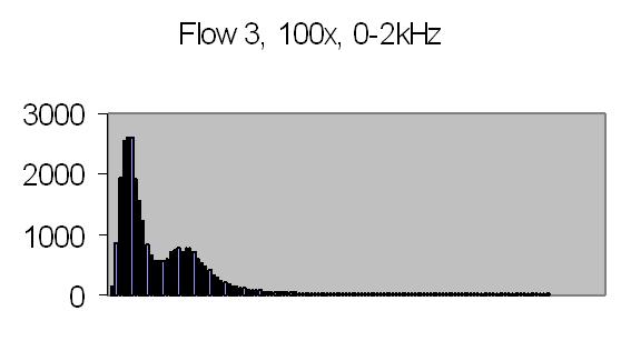
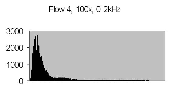
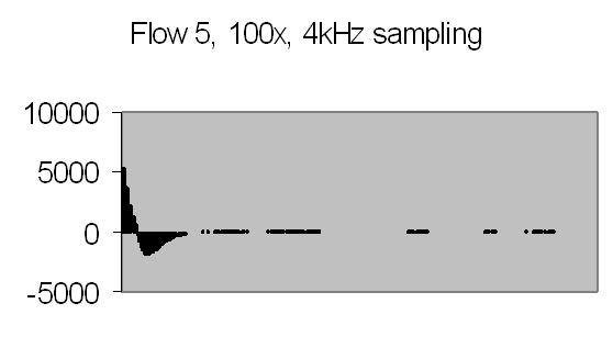
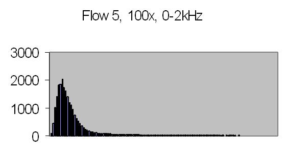
The energy spectra, like the power spectra, visualize the lower energy at higher frequencies. Figs. 29b and 30b show hardly any energy contribution from PALS at higher flows. Figs. 26b, 27b and 28b show two peaks: one from the Brownian movement, the second from PALS contribution. The latter peak is quite broad caused by fluctuations in uniform movement. It is difficult to produce a stable very slow flow by gravity.

The angle between the refracted crossing laser beams is 64.2 degree, Snell's law - 90 degree unrefracted (fig. 4). This angle results a spacing of ± 0.6 µm - equation (10). The computed particle velocity from flow 1 - a peak at ± 200Hz - becomes 0.012 cm/s. This is a very slow flow indeed! Air bubbles are not transported by such a slow flow. They collect in the tubing and glass capillary and cause the flow to stop sometimes. For ELS a more uniform movement is expected, thus resulting a narrow peak. Flow 2 shows a peak at ± 230Hz and flow 3 at ± 300Hz.

The sampling frequency of 4kHz is not randomly chosen. The autor is familiar with ELS equipment from Malvern Instruments Ltd, Malvern, UK. These ELS instruments apply a modulation frequency of 1000Hz to one of the mirrors (fig. 4). The modulation frequency gives an offset of 1000Hz to the result, enabling to find non-moving particles and determine the sign - positive or negative - of particle charge. The frequency shift found with these instruments will vary from 500Hz to 1500Hz. This fits precisely into the energy spectrum range - 0Hz to 2000Hz. Unfortunately, the lower energy contribution from higher frequencies prevents tests above 400Hz. However, it is proven that above DSP microprocessor autocorrelator application can cover the required range, providing 256 channels of autocorrelation. The limit depends on the FFT log2 requirement and sample frequency. The application blocks when 512 autocorrelation channels are set for 4kHz sampling frequency.

A typical measurement duration time for above autocorrelation experiments is 5 minutes. However, after 30 seconds the peak due to PALS is clearly visible. A longer duration time is taken to get a smooth autocorrelation function. Adding a 32-bit multiplicand from a 16x16-bit multiplication to the 64-bit autocorrelation channel causes unstable results just after start of measurement. The particle velocities computed are absolute. No calibration is required. The PALS measurement principle is based on physics. There are several ways to determine peaks within a (frequency) distribution.

Conclusion

The results are successful. It is possible to setup a DSP microprocessor autocorrelator to measure low uniform motion of suspended particles. The number of correlator channels is comparable to commercial autocorrelators and the required range is covered.

However, in comparison to commercial autocorrelators, presented DSP 16-bit fixed point µP autocorrelator can not be applied for particle sizing. It is too slow. It would be interesting to research faster DSP µPs to enhance performance to meet particle sizing requirements. At 20kHz sampling frequency 64 autocorrelation channels can be set up with C542 DSP µP. This corresponds to a 50µs sample time. A 120MHz C549 µP runs three times as fast, reducing sample time to ± 17µs. The number of 64 autocorrelation channels is already sufficient for most particle sizing applications. For polydisperse distributions the available autocorrelations channels can be split up to provide different sample times and autocorrelation functions. Further enhancement could be achieved with DSP 32-bit µPs. From 10µs and shorter sample times a DSP µP autocorrelator would become interesting for particle size experiments.

The results have shown that - for PALS/ELS applications - a phototransistor can be used instead of a photomultiplier. There are a few systems on the market (e.g. Malvern Instruments Ltd.) which use phototransistors to measure ELS dynamic light scattering as replacement for PMTs. It is rarely seen. From a manufacturing point of view, the combination of a phototransistor system and a DSP µP autocorrelator reduces the hardware cost to a fraction (!) compared to hardware cost of a PMT system with a traditional hardware digital autocorrelator.

For further research some recommendations can be given:

• Repeat tests with ELS equipment, and measure ELS sample standards
• Second analog input of AC01 can be used to measure static light scattering. This requires a parallel DC amplification of the phototransitor analog output. This will enable to measure I, the average intensity of scattered light
  By using an AC amplifier no information about average I is found. However, the advantage of AC amplification is that - equation (9)- the normalized offset `1' disappears and the autocorrelation measured is directly the required one. It also results the autocorrelation function decay to zero instead of to an offset.
• If a modulation of one of the mirrors is required (fig.4), the ramp signal (e.g. 1000Hz) can be simultaneously generated by the analog output of AC01.
• The phototransitor surface area of 25mm² is not required. The surface determines the light sensitivity, but in this application the pinholes (fig.4) used determine the minimum surface required. 1mm² will already be sufficient. The phototransistor should have maximum sensitivity for the laser wavelength.
• No specifications are known of used phototransitor from UDT Sensors Inc. To maximize sensitivity it is very likely that internal amplifier has been designed as a CCD (charged coupled device) circuit, integrating received energy. Such a CCD circuit could be designed for a separate photovoltaic sensor allowing greater flexibility in amplification and filtering.

The described PALS experiment was done in 1999. Today, it is possible to design a digital correlator into a single FPGA (Field Programmable Gate Array) IC device.

References

1. A Course in Digital Signal Processing, Boaz Porat, John Wiley & Sons, Inc. NY (1997). ISBN 0-471-14961-6.


2. Laser Light Scattering, Charles S. Johnson, jr. and Don A. Gabriel, Dover Publ. Inc. NY (1995) republication of the work originally published as Chapter 5 of Spectroscopy in Biochemistry (Vol. II). ISBN 0-486-68328-1.


3. Using the FFT, Anders E. Zonst, Citrus Press, Titusville FL (1995). ISBN 0-9645681-8-7.


4. Understanding FFT Applications, Anders E. Zonst, Citrus Press, Titusville FL (1997). ISBN 0-9645681-9-5.


5. Analog-Digital Conversion Handbook, 3rd edition, Analog Devices Inc., Prentice Hall, Englewood Cliffs NJ (1986). ISBN 0-13-032848-0.


6. Discrete Mathematics, T24211 Course, Open University of the Netherlands, Heerlen (1990).


7. Linear Algebra, T25211 Course, Open University of the Netherlands, Heerlen (1990).


8. Digital Signal Processing Applications (using the ADSP-2100 family), Analog Devices Inc., Prentice Hall, Englewood Cliffs NJ (1990). ISBN 0-13-212978-7.


9. TMS320C54x DSP Reference Set, Volume 4: Applications Guide. Texas Instruments, Custom Printing Company, Owensville, Missouri (1996).


10. Applied Fourier Analysis, Harcourt Brace College Outline Series, Hwei P. Hsu, Harcourt Brace College Publishers, New York (1984). ISBN 0-15-60169-5.


11. Mie Scattering Calculations: Advances in Technique and Fast, Vector-Speed Computing Codes, Warren J. Wiscombe, NCAR Technical Note, June 1979 (edited/revised August 1996), Boulder Colorado. Internet publication ftp.climate.gsfc.nasa.gov/pub/wiscombe.


12. Light Scattering by Small Particles, H.C. van de Hulst, Dover Publications, Inc., New York (1957, 1981). ISBN 0-486-64228-3.


13. Absorption and Scattering of Light by Small Particles, C.F. Bohren, D.R. Huffman, John Wiley & Sons, Inc., New York (1983). ISBN 0-471-29340-7.


14. Princles of Optics, Electromagnetic Theory of Propagation, Interference and Diffraction of Light, 6^th edition, Max Born & Emil Wolf, Cambridge University Press, Cambridge UK (1980). ISBN 0-521-63921-2.